Statistics with Resampling - T-Test

What is a T-Test?

When you want to see if a product is effective at doing what it promises, you might want to compare it to a baseline and see if it performes significantly better than that baseline. If you also happen to have a number estimate for the baseline, you can use a one-sample t-test. The most commonly taught t-test is the Student’s t-test and it tests how likely it is that the mean of the population is equal to the baseline (this is the null-hypothesis). It uses the equation \(t = \frac{sample_{mean} - baseline}{sample_{s.d.} / \sqrt{sample_{size}}}\) to calculate a so called t-score. You can then use a table to look what t-score is needed for a certain level of confidence that the null-hypothesis is not true, given your degrees of freedom. While this method works, I don’t find it very informative or enlightening. I prefer the resampling alternative.

T-Test using resampling

To do a t-test with resampling, this is the plan: I will take the sample data and the baseline. Then, I will take repeated samples from the sample data where a value is allowed to get picked twice. From these samples, I will calculate the mean. Based on these sample-means, I will then get a distribution of the sample mean and using that, I can determine the chance that the mean of the sample data is not the same as the baseline. For this example calculation, lets say that I want to test if a drink makes runners do better in a sprint competition. The average time without the drink is 15 seconds, which will be the baseline.

set.seed(14062020)
baseline <- 15
sample_data <- c(14.5, 13.5, 15, 15, 15.5, 14.5, 13.5, 15.5, 14, 14.5)
repetitions <- 1000
resampled_means <- rep(NA, repetitions)

for (i in 1:repetitions){
  new_sample <- sample(x=sample_data, size=length(sample_data), replace=TRUE)
  resampled_means[i] <- mean(new_sample)
}

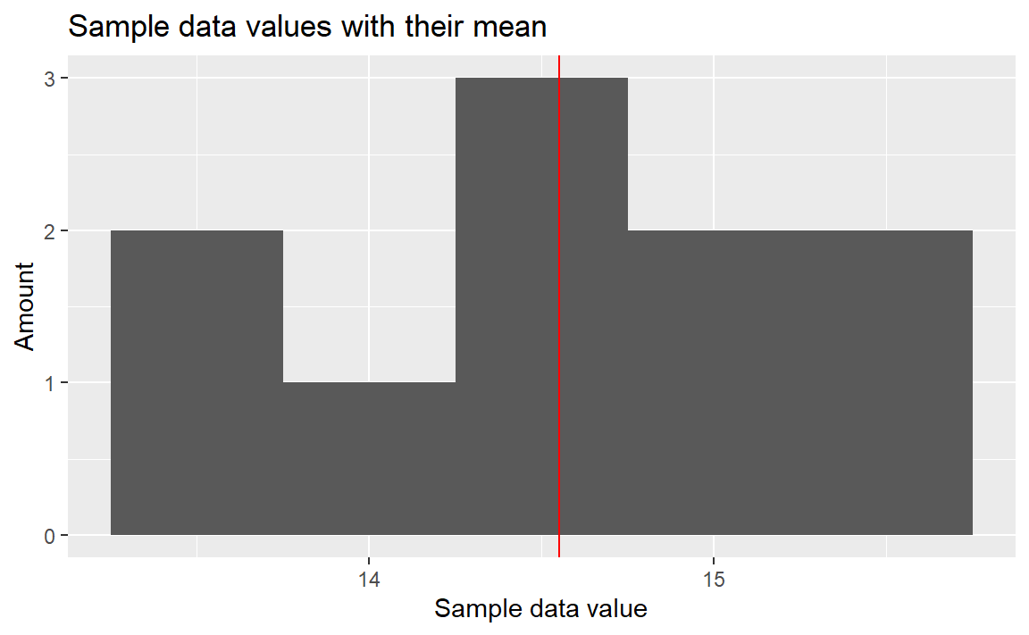
ggplot(mapping=aes(x=sample_data)) +
  geom_histogram(bins=5) +
  geom_vline(xintercept=mean(sample_data), color='red') +
  labs(title='Sample data values with their mean', 
       x='Sample data value',
       y='Amount')

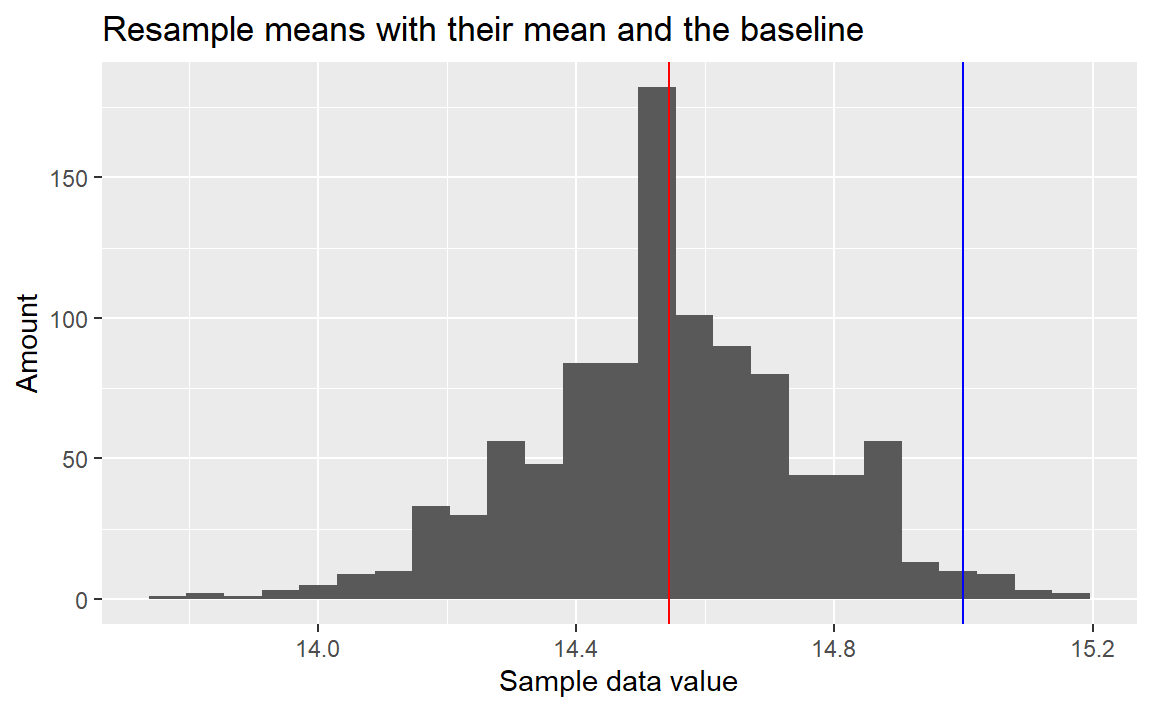
ggplot(mapping=aes(x=resampled_means)) +
  geom_histogram(bins=25) +
  geom_vline(xintercept=mean(resampled_means), color='red') +
  geom_vline(xintercept=15, color='blue') +
  labs(title='Resample means with their mean and the baseline',
       x='Sample data value',
       y='Amount')

sum(resampled_means >= baseline)/repetitions

## [1] 0.024

As you can see in the resample histogram, most means are smaller than the baseline than 15. If I calculate the exact number, which is the amount of values bigger than or equal to the baseline devided by the amount of means, I can see that only 2.4% of the resampled means is bigger than the baseline. This means that the chance that the null hypothesis is true is 2.4% and if we accept a chance of 1 in 20 of being wrong, we can reject the null hypothesis with a p-value of 0.05.

t.test(sample_data, alternative='less', mu=baseline)

## 
## 	One Sample t-test
## 
## data:  sample_data
## t = -1.964, df = 9, p-value = 0.04056
## alternative hypothesis: true mean is less than 15
## 95 percent confidence interval:
##      -Inf 14.97002
## sample estimates:
## mean of x 
##     14.55

As you can see in the results of the proper t-test, the estimate of 2.4% was not far of from the proper result of 0.04 and both come to the same conclusion