Statistics with Resampling - the Basics

Introduction

This blogpost and others that might follow are all based on what I learned from the great book Resampling: The New Statistics by Julian L. Simon. His book taught me everything that my Stat 101 class should have but did not and in a way that has shaped my thoughts about statistics. I will try to link to relevant chapters along the way where the ideas are covered in more detail.

What is resampling?

The idea of resampling is the following: instead of using mathematical formulas to answer questions, we draw random samples from a distribution or sometimes from a sample of data in order to answer the question. While this method still relies on the mathematical foundations of statistal distribution and their randomness, you get to see the moving parts more than when using formulas. Other names for this kind of method are bootstrapping, which focuses on just taking data from samples, and Monte Carlo simulations, which use probability distributions.

Resampling from a distribution

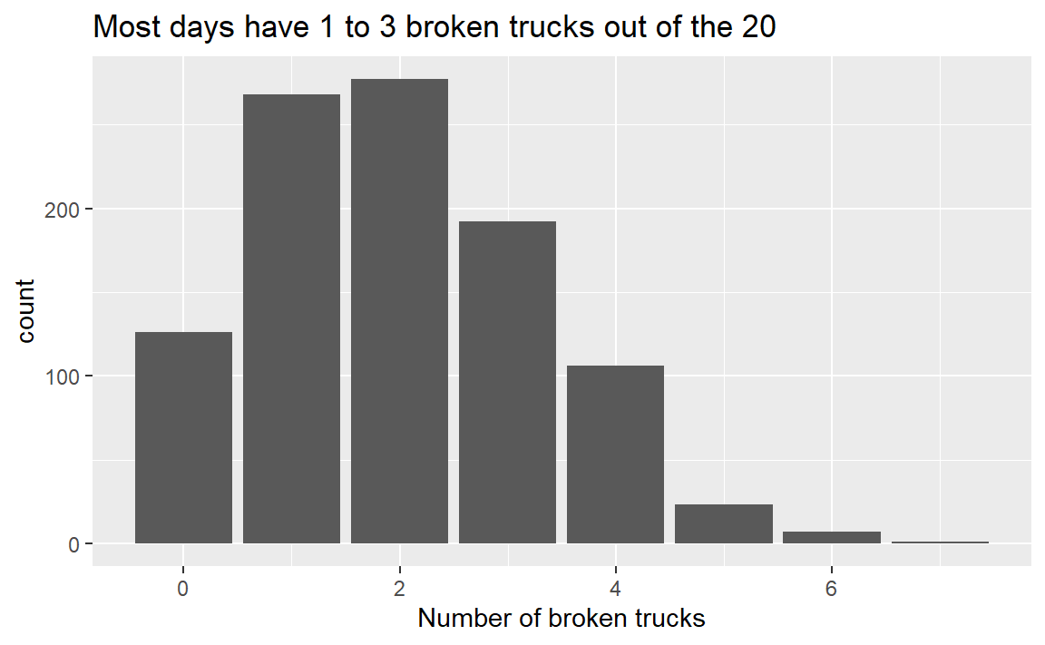
An example of a question we can answer using a distribution is about trucks breaking down. What is the chance that, for a company with 20 trucks and a 10% chance of each of the trucks breaking down, 4 trucks are broken down at the same time? We can answer this problem using different levels of abstraction. We can draw for each truck individually, for all 20 trucks at once or for all repetitions of the experiments. I will show the middle approach to showcase the resampling approach.

library(ggplot2) # Used for nice plots

## Warning: package 'ggplot2' was built under R version 4.0.5

set.seed(03062020) # This makes the random numbers reproducible
repetitions <- 1000
trucks <- 20
breakingchance <- 0.1
result <- rep(NA, 1000)

# This is equal to rbinom(repetitions, trucks, breakingchance)
for (i in 1:1000) {
   # If a truck breaks down, this results in a 1 and the sum is the amount of broken trucks
  result[i] <- rbinom(n=1, size=trucks,prob=breakingchance)
}
ggplot(data = data.frame(brokentrucks=result), 
       mapping = aes(x=brokentrucks)) +
  geom_bar() +
  ggtitle('Most days have 1 to 3 broken trucks out of the 20') +
  labs(x='Number of broken trucks')
 
print(sum(result >= 4)/repetitions)

## [1] 0.137

print(1 - pbinom(3, trucks, breakingchance))

## [1] 0.1329533

Figure 1: Good truck or bad truck

Resampling from a sample

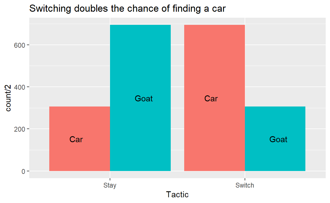
While this is a very limited sample, I think the problem and the mechanics do help with explaining the concept (the choice could also be modeled as a draw from a bernoulli distribution with a 33.3% chance of success). The problem we want to solve is the Monty Hall, or 3 doors problem. In a game, a contestant has to choose between 3 doors, 1 of which contains a car and the other 2 contain a goat. After the choice, the gamemaster will open 1 of the two doors and show a goat. The contestant gets the choice to switch, but should they?

set.seed(03062020) # This makes the random numbers reproducible
repetitions <- 1000 # Amount of times the experiment will be repeated
switch <- rep(NA, repetitions) # Prepare a vector for storing the results
stay <- rep(NA, repetitions) 

for (i in 1:repetitions) { # i is the index of the experiment we are at
  choice <- sample(c('goat', 'goat', 'car'), 1) # Initial choice
  if (choice == 'goat'){ # Contestant choose a goat, so will switch to the car
    switch[i] <- 'Car'
    stay[i] <- 'Goat'
  }
  else { # Contestant must have chosen the car
    switch[i] <- 'Goat'
    stay[i] <- 'Car'
  }
}

df <- data.frame(Tactic = c(rep('Switch', repetitions), rep('Stay',repetitions)),
                 Outcome = c(switch, stay))

ggplot(df, aes(x=Tactic, fill=Outcome)) +
  geom_bar(position='dodge') +
  geom_text(aes(label=Outcome, y=..count../2), stat="count", position=position_dodge(1), vjust='center', hjust= 'center') +
  ggtitle('Switching doubles the chance of finding a car') +
  theme(legend.position = 'none')

Figure 2: Should I stay or should I go?